
Written in Chinese, translated by Gemini 3.
If you have ever followed chess tournaments, played competitive ranked video games, or even glanced at Large Language Model (LLM) leaderboards, you have likely encountered scores like “1400,” “1800,” or “2500.” You are probably also familiar with the tiers these hidden scores determine: “Silver,” “Diamond,” or “Grandmaster.” You may have even heard the term “Elo rating.”
If you aren’t satisfied with the surface-level explanation that “higher scores simply mean better skills,” and instead want to understand “how these scores are calculated,” “why we rank based on them,” “the pros and cons of using them,” and “what the alternatives are,” then this article is for you.
In this article, the scores used to represent player levels in board games and esports systems will be collectively referred to as “Ratings.”
What is a Rating?
Many articles immediately throw the standard “Elo Rating” formula at you and then explain how to use it. I want to flip that approach: let’s first define the purpose of a rating, and then look back at how Elo’s mathematical model fulfills those needs.
Sorting by Ability
Ratings quantify “ability.” More precisely, they allow multiple competitors to be sorted based on their skill. The final result is the various leaderboards you see.
First, we must understand what kind of ability can be quantified by a rating, because not all abilities are easily ranked:
- The Incomparable: As the saying goes, “There is no first in literature, and no second in martial arts.” Assessing art or writing is subjective—beauty is in the eye of the beholder—whereas the outcome of a fight is objective and clear.
- Comparable but Unsortable: If we treat Rock, Paper, and Scissors as three players, they form a circular relationship of dominance. You cannot arrange them into a linear 1-2-3 order1.
Ratings are for abilities that are comparable and need to be sorted.
In different real-world scenarios, the method of “comparison” varies. In some competitions, there is a global method to score and sort all competitors simultaneously: think of the timing in a 100-meter dash or scores on a standardized test. However, in board games and combat sports, the only way to compare ability is local: “Head-to-Head outcomes.”
Ratings apply only to the latter. It is a method for converting the local results of “Head-to-Head” matches into a “Global Ability Ranking.”
An Ideal Rating: Win Rate
Now that we’ve clarified that the input is a history of “head-to-head results” and the output is a “global ranking,” let’s look at how to perform this conversion in an ideal scenario.
Suppose there are $N$ players. They play against every other player, determining a winner and a loser (let’s ignore draws for now). To reduce the factor of luck, each matchup is repeated $M$ times. After exhausting all $M\times N(N-1)/2$ matches, an intuitive and undisputed way to rank them is to sort by their respective number of wins. In other words, we determine ability based on sufficient win/loss data.
Since every player participates in the same number of matches, when $M$ is sufficiently large, the number used for sorting—the so-called Rating—approaches that player’s average win rate against the field.
This insight is crucial: The core of all rating algorithms is predicting some form of win rate.
In an ideal world, this win rate could be easily calculated after an infinite number of matches. However, reality is much harsher than this ideal:
- The number of players $N$ is not fixed. Newcomers join and veterans retire constantly, while the system must persist.
- Repeated matchups are insufficient. It is difficult to make $M$ large enough to eliminate luck when comparing two players.
- Ratings need to “accumulate.” We cannot wait for a massive batch of matches to calculate; updates should ideally happen after every game.
- Matchmaking is never truly uniform. In reality, we rarely force a Chess Grandmaster to play against a complete beginner.
A good rating system must estimate win rates as accurately as possible despite these confounding factors.
Practical Uses of Ratings
Ratings serve two main purposes:
Selection and Sorting. Whether it’s a hall of fame leaderboard or a tiered system for tournament qualification (like “Silver” or “Gold” ranks), when we need public, fair, and global decision-making, we need a relatively objective, absolute, and simple score for sorting and stratification—even if a player’s full competitive nuance cannot be captured entirely by these numbers. This is no different from a GPA or SAT score.
Skill Matching. This allows players to find opponents of similar skill levels—specifically, “matches where the win rate is around 50%.” This keeps the game engaging and provides an environment for players to learn and improve quickly. Purely random matchmaking would result in meaningless “stomps” (crushing victories or defeats). Go rankings and Esports ladders both operate on this principle.
You might immediately notice that “Skill Matching” does not actually require the global scores needed for “Selection and Sorting.” We could use any complex modern non-linear method (like a personalized recommendation system) to find a batch of opponents for Player $A$ against whom the local win rate $P(\text{win}|\text{vs A})$ is about 50%. We don’t strictly need opponents whose Ratings are close (which, in the ideal case above, implies their Global Win Rate $P(\text{win})$ is close to $A$’s).
If the distinction isn’t immediately clear, consider the case of “stylistic counters.” For example, table tennis player $A$ might be terrible at handling “choppers” (defensive backspin players). Therefore, when facing player $B$, who specializes in chopping but is weak in other areas, the two might have a 50/50 split, allowing $A$ to train against their weakness. However, since $B$’s overall skill is far below $A$’s, in a system that matches purely by Rating, the two would almost never meet.
Although a matching system built on local win rates offers a more flexible experience, the principle of competitive fairness often prevails. Because using a single score as the basis for both selection and matching is simpler and easier for the vast majority of people to understand, avoiding controversy, the Rating-based matching system has persisted in many modern online games.
So, What Exactly is a Rating?
In summary, a rating is essentially a win-rate prediction model squeezed through a tiny bottleneck:
flowchart LR
    n1["Historical Match Records"] --> n2["Player A's Rating"] & n3["Player B's Rating"] & n4["Player C's Rating"] & n5["Player D's Rating"]
    n2 --> n6(["Predict Win Rate: A vs C"])
    n4 --> n6

    n1@{ shape: procs}
    n2@{ shape: rounded}
    n3@{ shape: rounded}
    n4@{ shape: rounded}
    n5@{ shape: rounded}
It compresses all past “Win/Loss Records” into a single score per player, such that using the scores of any two players is sufficient to optimally predict the “Win Probability” of their match.
It is worth emphasizing again that “optimal” here is constrained by the condition that we can only use one score per side.
Deconstructing Elo
Having clarified the context, let’s examine how the classic Elo rating system implements these functions.
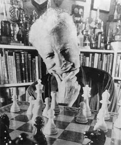
A bit of background: Arpad Elo (1903-1992) was a Hungarian-American physicist and a chess master. He invented the Elo rating system in 1960. It was first adopted by the US Chess Federation, spread quickly, and became the official FIDE (International Chess Federation) rating system in 1970.
FIDE titles correspond roughly to the following ratings:
- 2500+: Grandmaster (GM)
- 2400-2499: International Master (IM)
- 2300-2399: FIDE Master (FM)
Amateur ratings generally range between 1400 and 2200.2
Elo is also widely used in competitive video games. For context, in games like League of Legends, a “Diamond” tier might correspond to roughly 2000 MMR (Matchmaking Rating), while “Challenger” requires significantly higher scores.
Estimating Win Rate with Elo
First, let’s see how Elo ratings predict win rates. The core formula is elegant: if Player $A$ and Player $B$ have Elo ratings $R_A$ and $R_B$, the estimated win rate for $A$ is:
$$ \hat{P}(A \text{ wins}) = \frac{1}{1+10^{(R_B-R_A)/400}} $$The estimate for $B$ is symmetrical:
$$ \hat{P}(B \text{ wins}) = 1-\hat{P}(A \text{ wins}) = \frac{10^{(R_B-R_A)/400}}{1+10^{(R_B-R_A)/400}} = \frac{1}{1+10^{(R_A-R_B)/400}} $$Under the Elo model, the win rate between a pair of players is determined solely by the normalized difference in their ratings: $x=(R_B-R_A)/400$. This means absolute numbers like 1400 or 2200 have no inherent meaning; only the relative difference matters. The number 400 is just a convention to make the scores readable and standardized; it has no physical significance. If you added or subtracted an arbitrary constant to everyone’s score, or multiplied/divided them by a constant, it would not fundamentally change the Elo model’s behavior.
The function $f(x)=1/(1+10^x)$ simply maps the rating difference $x$ to a valid probability between $0$ and $1$:
- When $R_B=R_A$, both sides have a win probability of $1/(1+10^0)=1/2$.
- As $R_B-R_A$ approaches positive infinity $+\infty$, $A$’s win rate approaches $1/\infty$, i.e., $0$.
- As $R_B-R_A$ approaches negative infinity $-\infty$, $A$’s win rate approaches $1/(1+0)=1$.
With this formula, we can quickly estimate win rates in practice:
| Score Diff ($R_A - R_B$) | A’s Expected Win Rate |
|---|---|
| +800 | ~99% |
| +400 | ~91% |
| +200 | ~76% |
| +100 | ~64% |
| 0 | 50% |
Calculating Elo from Results
Now, let’s look at how Elo ratings are calculated from match history. If $A$ plays $B$ and $B$ wins, their scores update as follows:
$$ \begin{align*} R_A^{new} &= R_A+K(0-\hat{P}(A \text{ wins}))\\ R_B^{new} &= R_B+K(1-\hat{P}(B \text{ wins})) \end{align*} $$Here, $K$ is a parameter set by people, representing the maximum theoretical change in Elo rating for a single game. In chess, top-level tournaments typically use $K=16$, while tournaments for newer players might use $K=32$ to allow for faster adjustments. In the formula above, $0$ indicates $A$ lost, and $1$ indicates $B$ won. If it were a draw, both lines would use $0.5$. The sum of the changes for both sides is always zero—satisfying the requirements of a zero-sum game.
Finally, the most important property: The winner’s rating increase is discounted by their predicted win probability.
Assuming $K=32$:
- If $\hat{P}(B \text{ wins})$ was 99% (i.e., $B$ was rated 800 points higher than $A$), this victory gives $B$ only 0.32 points.
- However, if $\hat{P}(B \text{ wins})$ was 36% (i.e., $B$ was rated 100 points lower than $A$), this victory gives $B$ a substantial 20.5 points.
This means there is very little gain for a master crushing a novice (“smurfing”), while a dark horse achieving an upset is richly rewarded. In other words, the further the original prediction is from the result, the larger the update, correcting the prediction more aggressively for next time.
Newcomers with no match history are generally given an initial score between 1200 and 1500. Customs vary; some federations require a novice to play a small tournament first, calculating an initial score based on performance against rated opponents. A talented player with no prior record will rise quickly to their true level by defeating higher-rated opponents one by one (especially with the higher $K$ values often used in novice brackets).
flowchart LR
n2["Player A Current Rating"] --> n6(["Predict A vs B Win Rate"]) & n8["Player A New Rating"]
n4["Player B Current Rating"] --> n6
n6 --> n7["A vs B Match Result"] & n8
n7 --> n8 & n9
n6 --> n9["Player B New Rating"]
n4 --> n9
n2@{ shape: rounded}
n4@{ shape: rounded}
n8@{ shape: rounded}
n9@{ shape: rounded}
This forms the “ecological loop” of the Elo system. Estimating win rates before the match and updating scores after is so simple that players can even calculate it by hand at the venue.
Of course, if a player’s goal is to estimate win rates as precisely as possible, the Elo model is extremely primitive, even laughable: it assumes a single number (rating difference) is sufficient to predict the outcome! Obvious data that could improve prediction accuracy—like average K/D ratios in esports, blunder statistics in chess, head-to-head history, or recent form—are completely ignored. But Elo was never meant to be a hyper-precise prediction model; it is designed to compress the player capability determining victory or defeat into a single number.
In statistical and machine learning terms, this is called single-degree-of-freedom representation learning: extracting the essence (ability value) from raw data (win/loss records) via a predictive task (predicting win rates).
Statistical Interpretation of Elo
This section is intended for readers with a background in statistics or machine learning.
The Elo system is essentially a binary classification linear model (Logistic Regression) where player ratings act as the parameters. The parameters are optimized using Online Stochastic Gradient Descent (SGD) with Negative Log Likelihood (NLL) as the loss function.2
Let’s switch to standard mathematical notation for this section. Let $\bm{\theta}=(\theta_1,\dots,\theta_N)$ be the current ratings of $N$ players. The data for the next match (the $t$-th match) is $(\mathbf{x}_t,y_t)$, where:
- Feature vector $\mathbf{x}=(x_1,\dots,x_N)$ represents the match participants: $x_i=1$ means the $i$-th player is $A$, $x_j=-1$ means the $j$-th player is $B$, and all other $x_n=0$ where $n\neq i,j$.
- Binary target $y = 1$ means $A$ won, and $y = 0$ means $A$ lost (i.e., $B$ won; assuming no draws).
Without loss of generality, we change the base of the logarithm in the original Elo formula from $10$ to $e$ and remove the normalization factor of $400$. It becomes the Logistic Regression prediction for the probability $P(y=1|\mathbf{x})$ that $A$ wins:
$$ \hat{y}_t = \frac{1}{1+e^{-\bm{\theta}^\intercal\mathbf{x}_t}} $$Note that $\bm{\theta}^\intercal\mathbf{x}_t = \theta_i-\theta_j$. The loss function of the model is the standard Negative Log Likelihood:
$$ \mathcal{L}(y_t,\hat{y}_t) = -y_t\log{\hat{y}_t} - (1-y_t)\log{(1-\hat{y}_t)} $$The stochastic gradient update for the $t$-th sample is:
$$ \bm{\theta}^{(new)}=\bm{\theta}-\eta \nabla \mathcal{L}(y_t,\hat{y}_t) $$Where $\eta$ is the learning rate. Assuming $y_t=1$ (A wins), the update for $A$’s rating $\theta_i$ is:
$$ \begin{align*} \theta_i^{(new)} &= \theta_i-\eta \frac{\partial}{\partial \theta_i} \mathcal{L}(y_t,\hat{y}_t) \\ &= \theta_i+\eta \frac{\partial}{\partial \theta_i} (y_t\log{\hat{y}_t} - (1-y_i)\log{(1-\hat{y}_t)}) \\ % &= \theta_i+\eta \frac{\partial}{\partial \theta_i} \log{\hat{y}_t} \\ % &= \theta_i+\eta \frac{\partial}{\partial \theta_i} \frac{1}{1+e^{-\bm{\theta}^\intercal\mathbf{x}_t}} \\ &= \theta_i+\eta \frac{\partial}{\partial \theta_i} \log\frac{1}{1+e^{\theta_j-\theta_i}} \\ &= \theta_i+\eta (1-\frac{1}{1+e^{\theta_j-\theta_i}}) \\ &= \theta_i+\eta (1-\hat{y}_t) \\ \end{align*} $$The transition from the third-to-last to the second-to-last step utilizes the chain rule and the derivative properties of the Sigmoid function. The final result is exactly the score update formula mentioned in the previous section: $R_A^{new}=R_A+K(1-\hat{P}(A \text{ wins}))$.
So, simply put, the Elo rating system is just Online Logistic Regression calculated by hand.
Beyond Ratings
We now know where rating systems are useful and have traced the logic behind the classic Elo system. The obvious next question is: Can we do better?
If “Skill Matching” can be separated from “Sorting/Selection,” the “single degree of freedom” bottleneck at the center of the rating model can be loosened, allowing for more flexible and complex modeling possibilities.
Elo uses the simplest binary classification model. We could swap this for a large neural network, using black-box encoders like RNNs, CNNs, or Transformers to scrutinize match history and output much more precise win rate predictions. Similarly, we could employ cutting-edge adaptive gradient optimizers to update parameters after every match—parameters that would be far more complex than a single rating per person and thus harder to interpret. We could represent a player’s ability with a multi-dimensional vector rather than a single value, visualize them with hexagonal “radar charts,” and attribute the gap between predicted and actual results to specific dimensions, revealing latent weaknesses for targeted training. We could even abandon the single, short-sighted standard of current win/loss and introduce long-term positive metrics—such as tendency for cooperation in online team matchmaking or a player’s rate of improvement. These complex “Multi-Ability to Multi-Outcome” models could customize matchmaking for players in different contexts, helping both sides achieve effective improvement or simply have more fun.
However, for public selection and leaderboard generation, standard ratings are sufficient. The Elo system is simple to calculate and transparent. Even with many later derivatives (like Glicko3, which introduces a measure of rating volatility; or TrueSkill4, which introduces team contributions and consistent Bayesian updates), it does not feel obsolete.
But we must remain wary of the impulse to “over-interpret” a linear leaderboard. Often, the abilities or traits we care about are not sortable. From Rock-Paper-Scissors to university rankings, things in life are usually far more complex than a column of numbers.
As Professor Elo lamented in a 1982 interview5:
Sometimes I think I’ve created a Frankenstein’s monster with this system because some of the young players become just like race track habitues who never really see a race; all they do is peruse the tote sheets.
Mathematically, this comparison relationship lacks transitivity: if $a<b$ and $b<c$, it does not necessarily imply $a<c$. ↩︎
https://en.wikipedia.org/wiki/Glicko_rating_system ↩︎